Welcome to the Wildfire Vulnerability Explorer

This website was designed to allows users to explore a set of spatially explicit models developed for the Sensor Technology for Improved Wildland Urban Interface (WUI) Fire Resilience project. The goal of this project is to design, develop, and deploy a hybrid temperature sensor network to help support post-fire assessments of water infrastructure damage. The models presented on this website serve to support this effort by identifying communities that are likely to be vulnerable to water contamination exposure following a large scale fire event. These models estimate vulnerability based on three primary factors: probability of water contamination, socioeconomic sensitivity, and adaptive capacity (i.e., a community's ability to adjust to, and recover from, water infrastructure damage). The relationship among these factors can be summarized as follows:

Vulnerability = Probability of Water Contamination + Socioeconomic Sensitivity - Adaptive Capacity

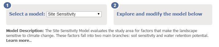
For more information, click on the "Learn About the Models" tab, or click on the "Explore the Models" tab to jump right in.

Project Information

To learn more about the project, including a list of team members and contact information, visit the Project Website.

Funding for this project was provided by the Alfred P. Sloan Foundation.

A Primer on EEMS & Fuzzy-Logic

The models presented on the next tab were created using the Environmental Evaluation Modeling System (EEMS), a fuzzy-logic modeling system developed by the Conservation Biology Institute (CBI). Simply put, fuzzy-logic allows you to assign shades of gray to thoughts and ideas rather than being limited to the binary (true/false) determinations of traditional logic. It is this concept of "partial truth" which allows fuzzy-logic models to more accurately capture and resemble human patterns of thought.

About the Vulnerability Models

Clicking on the "Explore the Models" tab brings up an interactive model diagram on the left and a map display on the right. As described above, the final proposition being evaluated in each model is "High Vulnerability to Water Contamination Exposure". The final values in each reporting unit indicate how true or how false this statement is.

• Red areas in the map show where the final proposition is true (on a gradient from 0 to 1).
• Blue areas in the map show where the final proposition is false (on a gradient from 0 to -1).

Proposition: High Vulnerability to Water Contamination Exposure
Totally False	Somewhat False	Somewhat True	Totally True

As you explore the model diagram, you'll see that the level of vulnerability is based on three main branches:

1. Probability of Water Contamination (based on the likelihood that contamination levels will exceed the maximum allowable contamination level (MCL))
2. Socioeconomic Sensitivity (based on demographic data extracted from 2010 CENSUS blocks and block groups)
3. Adaptive Capacity (based on a community's ability to adjust to, and recover from, infrastructure damage)

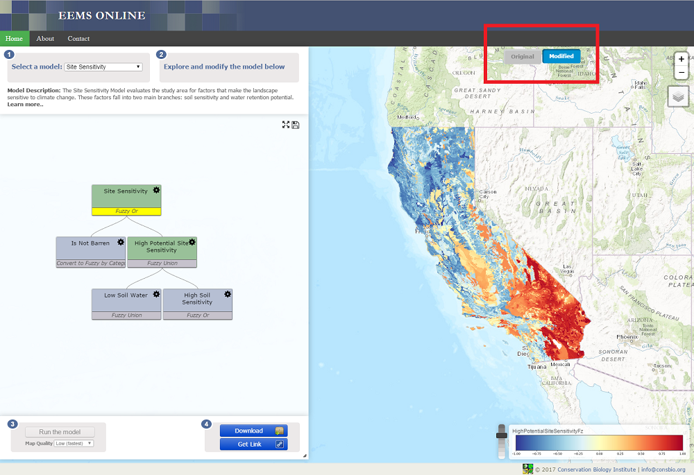
These three branches get combined using a "Weighted Union". A "Union" in fuzzy-logic simply takes the mean average of the inputs. This operator is used when all of the inputs should exert an influence on the result. A Weighted Union is similar to a Union, except that it allows weights to be applied to the inputs. It's used when each input should exert an influence on the result, but to a varying degree. In the vulnerability models, each of the three branches listed above contribute to the level of vulnerability, but the risk of water contamination and socioeconomic sensitivity are weighted higher (have more influence) than adaptive capacity.

Download the Data (Final Model Outputs)

Santa Rosa (With Adaptive Capacity)
Santa Rosa (Without Adaptive Capacity)

Paradise (With Adaptive Capacity)
Paradise (Without Adaptive Capacity)

Model Inputs

The input data used to create the vulnerability models were derived from two primary sources, described below.

Probability of Water Contamination

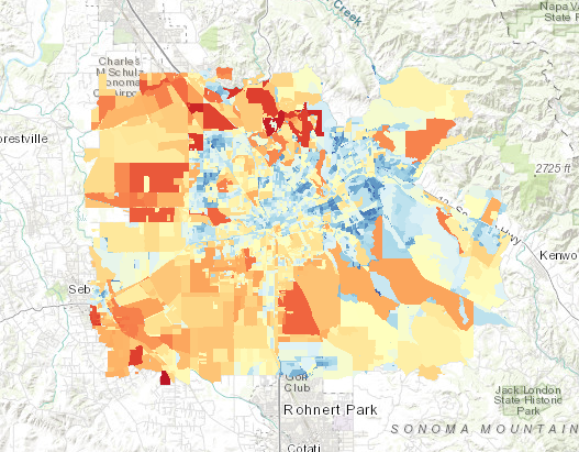
The water contamination datasets used in these models were created by Dr. Andres Schmidt at Oregon State University. Grid cell values in these 30m rasters provide absolute probabilities of drinking water contamination exceeding the State of California MCL for Benzene (1 µg/L) for water samples from the water distribution system after a collocated wildfire event.

To create these datasets, Bayesian regularized neural network ensembles were trained using high-resolution data layers comprising topography, soil properties, landcover, vegetation, meteorological parameters, fuel load, and infrastructure data. In combination with post-fire water samples, the input data was used to map the risks of MCL exceedance to the values observed in the cities of Santa Rosa, CA and Paradise, CA.

Once the model is optimized to reproduce the training data and generalize well enough to also model new data (not included in the training process) with sufficient accuracy, the model is applied to the entire model domain with a 30 m x30 m resolution as illustrated in figure 1. Several models can be averaged to build an ensemble result at each grid cell point which in practice often increases the generalization capabilities of the models and hence, their accuracy. The results for the risk of water contamination shown as part of the EEMS model give the conditional probability that post fire water samples exceed the California MCL for benzene in drinking water (1 µg/L) after a potential fire.

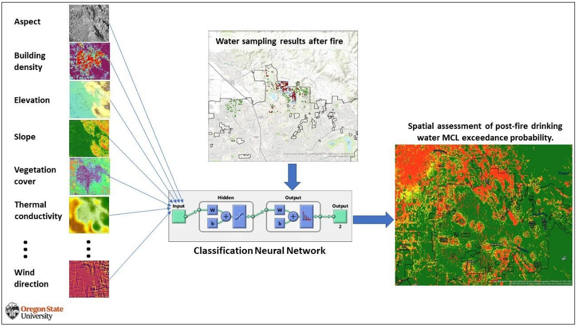
Input data variables used to calculate the risk were aggregated to 30 x 30 m spatial resolution. For the topographic data layers, we used the 30 m NASA Shuttle Radar Topography Mission dataset (SRTM) version 3.0. Aspect values were calculated using the ESRI ARCGIS Surface Parameters tool with adaptive neighborhood selection and quadratic surface functions fitted around each grid cell. Vegetation fuel load was quantified through landcover type, percentage vegetation cover, and vegetation height. We used the LANDFIRE 2016 Remap (LF 2.0.0) for existing vegetation height (EVH) and percentage vegetation cover. The Multi-Resolution Land Characteristics Consortium (NLCD 2016) dataset was used for landcover type classification.

The locations of buildings were taken from the 2018 Microsoft Building Footprint data that was created from satellite and aerial imagery using the ResNet34 deep neural network. The spatial values for contents of clay, silt, and sand, as well as soil bulk density were downscaled using the WoSIS and SoilGrids datasets publicly provided through soilgrids.org. Locations of fire stations were obtained from the Homeland Infrastructure Foundation-Level Data database (HIFLD). Wind fields were then downscaled with WindNinja (ver. 3.7.2) to account for topography and surface roughness and obtain the 30 m resolution wind fields for the two model domains. The thermal conductivity of soil has a strong effect on the resulting belowground temperature and, hence, the heat-related pipeline damage from aboveground fire potentially causing deformation, melting, and heat-induced release of contaminants in belowground water pipes. Using the soil data from the SoilGrids repository in combination with average soil moisture values during the months of the fire occurrences from the TerraClimate database. Post-fire water samples for network training were collected and provided by the Paradise Irrigation District.

For additional information on the probability of water contamination data, download the journal article published in Machine Learning for Applications (Volume 7, 15 March 2022), which can be accessed by clicking the link below.

Download the Journal Article

Predicting conditional maximum contaminant level exceedance probabilities for drinking water after wildfires with Bayesian regularized network ensembles

Download the Data

Georisk Continuous (Generalized), Paradise, CA
Georisk Continuous (Generalized), Santa Rosa, CA

Socioeconomic Sensitivity & Adaptive Capacity

The socioeconomic sensitivity datasets used in these models were compiled by Dr. Jenna Tilt at Oregon State University. These datasets include Census Block, Blockgroup and Paradise Parcel data to describe the socio-economic, landuse, and housing characteristics of each study area. This information is used in each model to identify areas (e.g. Census Blocks) that have high population (e.g. low income, education) or land use sensitivity (e.g. multi-dwelling units, critical facilities) and may be more vulnerable to natural hazards.

Adaptive capacity refers to a community's ability to adjust to, and recover from, infrastructure damage. For the Santa Rosa study area, the adaptive capacity calculation is based on a subset of the socioeconomic variables (wealth, housing characteristics, and household characteristics). For the Paradise study area, this estimate is based on the number of pre-fire backflow devices installed per capita within each Census block (these data, provided by the Paradise Irrigation District, are private and may only be used for visualization purposes with the Wildfire Vulnerability Explorer).

2010 Census Block data was retrieved through the IPUMS National Historical GIS: Steven Manson, Jonathan Schroeder, David Van Riper, Tracy Kugler, and Steven Ruggles. IPUMS National Historical Geographic Information System: Version 15.0 [dataset]. Minneapolis, MN: IPUMS. 2020. http://doi.org/10.18128/D050.V15.0.

2012-2016 American Community Survey data was retrieved through the IPUMS National Historical GIS: Steven Manson, Jonathan Schroeder, David Van Riper, Tracy Kugler, and Steven Ruggles. IPUMS National Historical Geographic Information System: Version 15.0 [dataset]. Minneapolis, MN: IPUMS. 2020. http://doi.org/10.18128/D050.V15.0.

City of Santa Rosa parcel information (2016) was provided by the City of Santa Rosa and Sonoma County Assessor Department.

Town of Paradise parcel information (2018, before the Camp Fire) was provided by Butte County Assessor Department.

Download the Data

Socioeconomic Sensitivity (CENSUS Blocks), Paradise, CA
Socioeconomic Sensitivity and Adaptive Capacity (CENSUS Blocks), Santa Rosa, CA

Exploring the Model Diagram

• Click on a box (node) in the model diagram to display the corresponding layer in the map.
• Click in the map to see the fuzzy (truth) values calculated for each node (these values allow you to determine which factors have the most influence on the things above it).

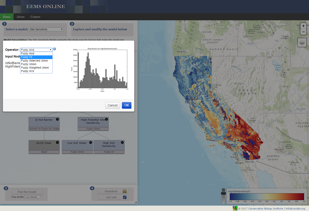
The nodes at the very bottom of the tree (the dark gray boxes) represent the original input data. When building a model, all of the input data, regardless of type (ordinal, nominal, or continuous), are first converted into fuzzy values between -1 (false) and +1 (true). This is typically done by setting a True Threshold (a value that indicates when a proposition becomes totally true) and a False Threshold (a value that indicates when a proposition becomes totally false). Input values between these two thresholds receive a floating point value between -1 and +1 based on a linear interpolation.

Once all of the input data has been converted into "fuzzy space", the resulting nodes are combined using fuzzy logic operators (e.g., AND, OR, UNION). The operator used to combine a set of input nodes appears at the bottom of the output node. Refer to the table below for a list of available operators and a description of what they do.

Selecting a Different Model

The Santa Rosa model will be selected by default. To select a different model, click on the dropdown menu labeled #1 in the control panel shown below. A short description provides some basic background information about the model. Click on the "Learn more" link for additional information.

Making Changes to a Model (Advanced)

Clicking the gear icon on any node brings up a dialog box that allows you to make changes to the operator, or change the operator to a different operator (Fig 2). This allows advanced users to explore different ways of combining the data, to experiment with different weights, etc. A histogram will also appear to the right of the operator selection menu which will show the distribution of data for the current node. The Y-Axis indicates the number of reporting units that have the corresponding value on the X-Axis. The available options will vary depending on the node's current operator.

Available Operators

The table below lists the available operators, along with the type of data expected as input and a brief description:

Operator	Input Data	Description
AND	Fuzzy	Finds the AND value of the inputs (minimum value).
		(previously OrNEG in EEMS version 1.0)
CONVERT TO FUZZY	Raw	Converts a field's values into fuzzy values.
Convert To Fuzzy Category	Raw	Converts a field's values into fuzzy values by using the user defined category values and matching fuzzy values. Input values that are not in the user defined categories are assigned the user-defined default fuzzy value.
EEMS Convert To Fuzzy Curve	Raw	Converts a field's values into fuzzy values for EEMS (Environmental Evaluation Modeling System), using linear interpolation between user defined points on an approximation of a curve.
Difference	Raw	Computes the difference sum for each row of the inputs.
EEMS EMDS And	Fuzzy	Fuzzy logic operator for EEMS (Environmental Evaluation Modeling System). Finds the EMDS AND value of the inputs. The formula is min + [(mean - min) * (min + 1) / 2]
Max	Raw	Finds the maximum for each row of the input fields.
Mean	Raw	Finds the mean for each row of the input fields.
Min	Raw	Finds the minimum for each row of the input fields.
Not	Fuzzy	Logical NOT for fuzzy modeling. Reverses the sign of values of the input field.
OR	Fuzzy	Finds the truest value of the inputs (maximum value).
SELECTED UNION	Fuzzy	Finds the union value (mean) of the specified number of TRUEest or FALSEest inputs.
SUM	Raw	Computes the sum of the inputs.
UNION	Fuzzy	Finds the union value of the inputs (mean value).
Weighted EMDS And	Fuzzy	Finds the weighted EMDS AND value of the inputs. The formula is min + [(mean - min) * (min + 1) / 2] where the mean is weighted.
WEIGHTED MEAN	Raw	Finds the weighted mean for each row of the input fields.
WEIGHTED SUM	Raw	Finds the weighted sum for each row of the input fields. Multiplies each field by its weight before adding. Like a weighted mean without the division.
WEIGHTED UNION	Fuzzy	Finds the weighted union (mean) for each row of the input fields.
XOR	Fuzzy	Finds the fuzzy EXCLUSIVE OR value of the inputs by comparing the two truest values. If both are fully true or fully false, false is returned. Otherwise it applies the formula: (truest value - second truest value) / (full true - full false)

Choosing an Operator

EEMS presents the user with choices for many operators and finding the right one can be confusing at first. The guidelines presented here will help you choose the right operator, but remember, sometimes it is best to experiment with several choices to make sure the operator you choose is appropriate for your model.

EEMS has operators designed to work on data before they are converted into fuzzy numerical space (i.e. when they are still in raw space) and those designed to work on data after they are converted into fuzzy space (see the above table). A user should respect that distinction. Using a non-fuzzy operator on fuzzy data can produce a result that falls outside the -1 to +1 continuum of fuzzy space. Doing this produces an invalid model.

Weighted Sum

The operators used in raw space are for the most part pretty straightforward. However the Weighted Sum operator merits a discussion. A Weighted Sum takes two or more inputs, and multiplies each of them by a weight before adding them. It has proven especially valuable with combining data of very similar types into one result that is then converted into fuzzy space. For example, if you were evaluating a region for intactness, the negative impact of paved roads might be considered similar to but greater than that of dirt roads. Their effects are additive, but a sum operator is not available in fuzzy space. To apply the Weighted Sum operator you might provide a weight of 1 to the paved road density and a weight of 0.5 to the dirt road density. In models that have done this, the result has been labeled “Effective Road Density.”

And, Or, and Union

And, Or and Union are the most common EEMS operators used. The choice between And, Or, and Union depends on the relationship of the input data to the question you are asking. Or returns the highest fuzzy value of any of the inputs, it is appropriate when any of the inputs is sufficient for your desired outcome. For example if you were evaluating a region in which three critically endangered species were present in some locations, you could use an Or to combine presence of species A, presence of species B, and presence of species C into high preserve value. The presence of any of the three species would cause a map reporting unit to have a high fuzzy value. And is used when all inputs are necessary for the result to be high. For instance, if both habitat for and presence of a species of interest were required to consider a location as a preserve, you could combine species presence and habitat density with an And to produce high preservation value. And chooses the lowest fuzzy value of the inputs so that high fuzzy values for both conditions are necessary to yield a high fuzzy value for the result. Union takes the mean of the input values. Union allows each input to exert an influence on the result. If all inputs have a high value, the result will have a high fuzzy value; if all have a low value, the result will be low. If some are high and some are low, the result will be somewhere in between. Going back to our preserve example, we know if the species is present, the location has value as a preserve. If the habitat is present there is some value, too. If they are both present then the value is the highest. Union will yield that result. A Weighted Union is similar to Union, except that it allows a weight to the inputs. In our preserve example, if habitat density is more important than species presence (for instance in an area where remnant populations are under stress and habitat has been restored in areas where the species has not been able to recolonize) then you could provide a greater weight to habitat density.

Selected Union

The Selected Union represents a combination of Or (or And) and Union. Consider a study area that includes many different types of habitat, for example, a basin and range terrain. Some species of concern are found in valleys, others inhabit the foothills, and others the high mountains. What if there are 30 species of concern? The more species of concern in a location, the more valuable the location, but nowhere are they all found together. The Selected Union allows for the evaluation of such a study area. With the Selected Union, you choose a number of the truest (or falsest) of inputs to evaluate. In the basin and range example, you might choose five. A location with a high density of five (or more) species of concern would have a high fuzzy value for high species diversity. As the density of species of concern falls, so does the fuzzy value for high species diversity. A Selected Union with a parameter of 5 Truest would do just that. It performs a Union operation on the five inputs with the highest fuzzy values.

Running the Model

You may specify any number of changes to the model. Operators that have been modified will be highlighted in yellow. Once you are satisfied with your changes, click the "Run the model" button labeled #3 on the EEMS Online Control Panel. The model run may take anywhere from several seconds to several minutes to complete, depending on the complexity of the model and the spatial extent and resolution of the input data.

Once the model run is complete, the changes will be reflected in the map. The buttons above the map allow you to change the map display between the original version and the modified version (shown below).

Once you have conducted a model run, you have the option of either making additional changes to the model and rerunning it, or, if you are satisfied with the results, you can click the Download button to download the output and associated model content, or push the Get Link button which will allow you to share the modified model or access the modified model through EEMS Online at a later time.

Model Inputs

This section describes the data and methods used to create the inputs to the EEMS fuzzy logic model.

Probability of Water Contamination

The information presented in this section is a summary of a journal article published in Machine Learning for Applications (Volume 7, 15 March 2022). Click on the link below to open the article in a new tab.

Predicting conditional maximum contaminant level exceedance probabilities for drinking water after wildfires with Bayesian regularized network ensembles

Many contributing factors and processes that can cause the post-fire contamination of drinking water in water distribution systems (WDS) are partially unknown or corresponding data unavailable. Processes such as the water distribution system-wide state of pressure, flow, and temperature in a complex pipe network across a town are unknown, except for certain main valves and control points. Furthermore, parameters change during wildfires when firefighting efforts or damaged pipes and associated pressure drops change flow rates and directions at one or many points of the distribution system.

Furthermore, current wildfire models do not allow for modeling burn probability or fire behavior in built-up areas due to a current lack of fuel models for such structures. Sections of built-up areas containing numbers of structures that can be close to burnable vegetation are currently classified as non-burnable in fuel layers of fire models. Hence, using a deterministic process model for spatial predictions of post-fire contamination risk with available sampling data and knowledge of processes, is currently unfeasible. For the spatial analyses here, we use a machine learning approach with pattern recognition networks that have SoftMax classification output layers to spatially predict conditional probabilities of drinking water contamination in WUI areas after fire affected the structures and the surrounding areas. We use analytical results of post-fire water samples, topographic factors, landcover data, information about infrastructure, and physical soil properties in combination with Bayesian regularized neural networks building ensemble models that predict conditional probabilities for benzene levels in WDS exceeding the maximum contaminant level (MCL) for benzene. Benzene is considered a carcinogen and poses a severe health threat to humans if consumed in high concentrations. While other contaminants were found in WDS water samples after wildfires, benzene was chosen as a representative Volatile organic compound because of its abundance in post-fire water samples in Santa Rosa and Paradise, California.

Using the water samples that were collected in any study area after the wildfire, the parameters of the neural networks are iteratively optimized to map the input data on the target data (i.e., the contamination status of post-fire water samples at each point).

Once the model is optimized to reproduce the training data and generalize well enough to also model new data (not included in the training process) with sufficient accuracy, the model is applied to the entire model domain with a 30 m x30 m resolution as illustrated in figure 1. Several models can be averaged to build an ensemble result at each grid cell point which in practice often increases the generalization capabilities of the models and hence, their accuracy. The results for the risk of water contamination shown as part of the EEMS model give the conditional probability that post fire water samples exceed the California MCL for benzene in drinking water (1 µg/L) after a potential fire.

Socioeconomic Sensitivity This socioeconomic sensitivity data identifies areas (e.g. Census Blocks) that have high population (e.g. low income, education) or land use sensitivity (e.g. multi-dwelling units, critical facilities) and may be more vulnerable to natural hazards. These data were derived from Census Block, Blockgroup, and Paraadise Parcel data.

Oregon State University (Dr. Jenna Tilt) compiled this dataset. 2010 Census Block data was retrieved through the IPUMS National Historical GIS: Steven Manson, Jonathan Schroeder, David Van Riper, Tracy Kugler, and Steven Ruggles. IPUMS National Historical Geographic Information System: Version 15.0 [dataset]. Minneapolis, MN: IPUMS. 2020. http://doi.org/10.18128/D050.V15.0 2012-2016 American Community Survey data was retrieved through the IPUMS National Historical GIS: Steven Manson, Jonathan Schroeder, David Van Riper, Tracy Kugler, and Steven Ruggles. IPUMS National Historical Geographic Information System: Version 15.0 [dataset]. Minneapolis, MN: IPUMS. 2020. http://doi.org/10.18128/D050.V15.0 Town of Paradise parcel information (2018, before the Camp Fire) was provided by Butte County Assessor Department.

Adaptive Capacity Adaptive capacity refers to a community's ability to adjust to, and recover from, infrastructure damage. For the Santa Rosa study area, the adaptive capacity calculation is based on a subset of the socioeconomic variables (wealth, housing characteristcs, and household characteristics). For the Paradise study area, this estimate is based solely the number of pre-fire backflow devices installed per capita within each Census block.

Drag n' Drop a CSV

You can drag and drop a CSV file containing lat/lon coordinates directly into the map. Clicking on any of the points will display all the values in the CSV for that point, as illustrated below. This allows you to examine sensor data, water contamination data, first responder data, etc., in relation to the EEMS model results in order to help with pre-fire planning or post-fire recovery efforts.

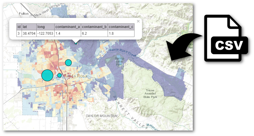
The CSV file should be structured as follows:

There are a few requirements to be aware of:

1. Lat/Lon values should be in WGS84.
2. The first three fields in the CSV file must be as follows: an ID field, a Latitude field, a Longitude field. Any number of attribute fields may follow.
3. The CSV must include field headers, but the header names can be whatever you wish (e.g., the ID field could be called ID or OID or PointID, and the latitude field could be called Lat or Latitude or Y, etc.)
4. The size of the points will reflect the value in the first "Var" field (i.e., the field after the longitude field). For that reason, your first "Var" field must contain numeric values (integer or float).

That's it! Once you have a CSV that meets the requirements above, simply drag it into the map.